Home Credit Default Risk

Abstract

Loans are important to lenders and borrowers. It is important to identify the risky behaviors of clients and make educated decision. This paper is built on an end-to-end machine learning case study for predicting the defaulting risk associated with a borrower. The paper highlights on the exploratory data analysis of the datasets, feature engineering and machine learning modeling techniques and assess the results of these models.

1. Introduction

There has been a significant increase in the banking industry recently in which the unbanked population who are not privy to financial literacy are discriminated against when applying to loans. This means there’s an inequity in the field of loan granting that needs to be remedied. Our objective is to predict the likelihood of loan repayment to better distribute loans. We came across a dataset on Kaggle from HomeCredit whose mission is to broaden financial inclusion for unbanked populations.

1.1 Background

The dataset consisted of seven different sheets: current application, bureau balance, credit card balance, installments, cash balance and previous installments. The main objective is to identify the potential Defaulters based on the given data about the applicants. The probability of classification is essential because we want to be very sure when we classify someone as a Non-Defaulter, as the cost of making a mistake can be very high to the company. Our goal was to utilize important features from these sources to identify which would be key in the resultant machine learning model. Our methodology included cleansing the data, visualizing various elements to better understand it, feature selection, model fitting, and derive our final conclusions.

Since the dataset was created for a datathon, the testing data did not include the labeled response. Therefore, we decided to create a 70/30 split on the training set in order to test the accuracy of the model.

2. Methods

2.1 Data Processing

Data preparation is integral to deriving clear and accurate results from a machine learning model. There are specific properties we noted when taking a deep dive into the data. It was incredibly dense, spanning across ~450 columns in total and ~307,000 rows. There were inconsistencies in the data types within the columns as well meaning it was heterogeneous in nature. It was also time-varying and there were unbalances in some of the responses that required cleansing. The following flow was utilized to understand the scope of the data and determine which predictive model would be best.

2.1.1 Data Exploration

We first hypothesized which features may be most important in determining the likelihood of loan repayment. Working with a few, we derived the following:

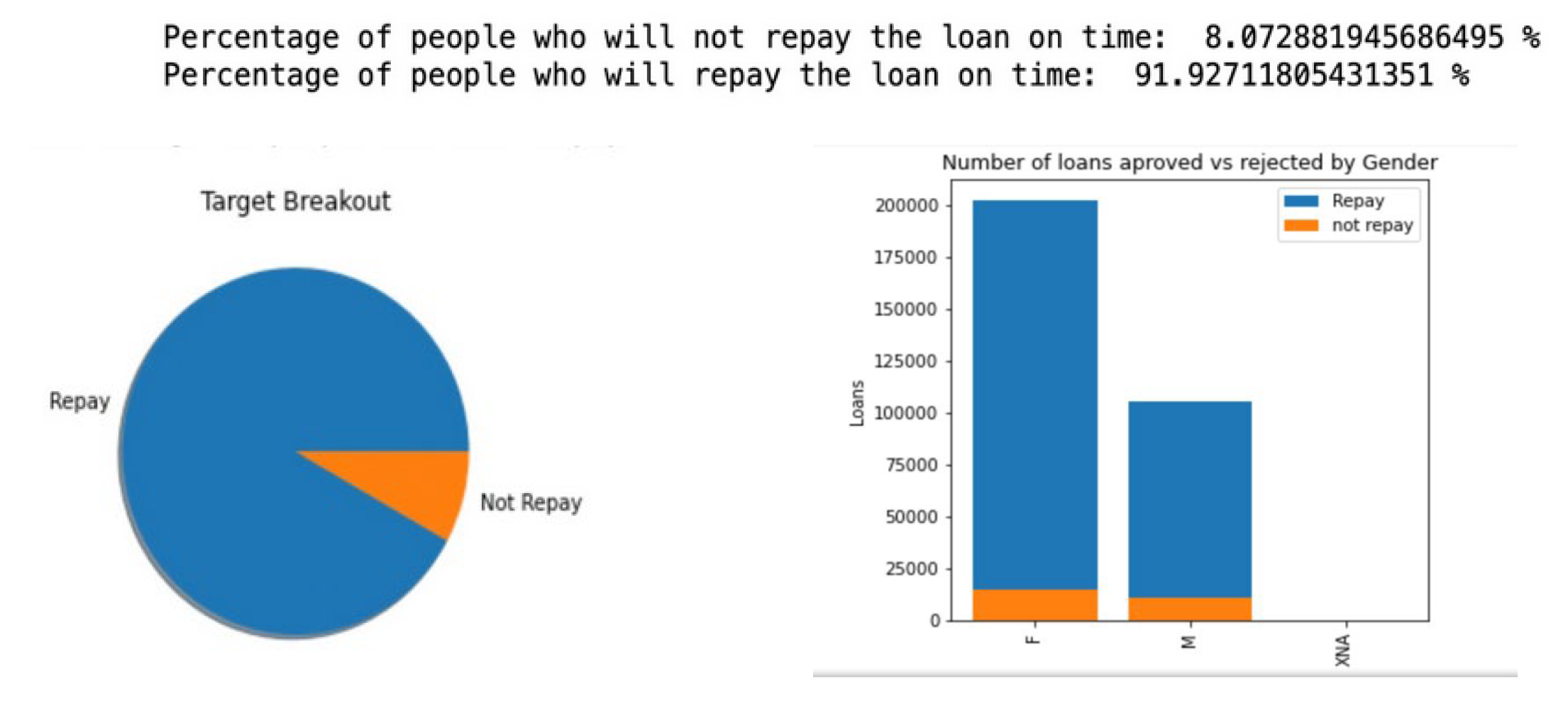
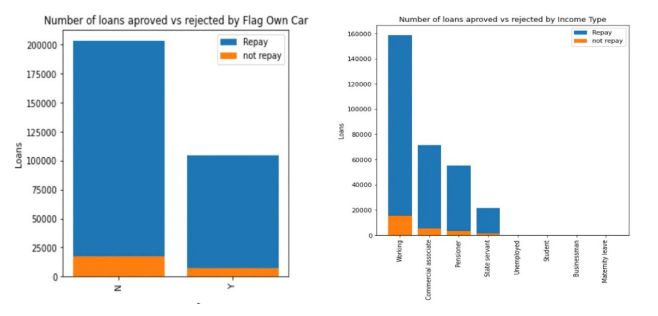
We began by looking at a high-level scale of metrics to gauge what our overall responses might look like. As you can see, the percentage of people who don’t pay back their loan was very small, so it was important to identify the correct model and execute accurate feature selection to isolate the variables most impact likelihood of repayment. Here are some breakdowns of main factors we initially thought would strongly influence the model. Again, we see an even dispersion of the target across all groups of the factors observed. However, we believed that car ownership may be a strong indicator that an ability to pay off a car loan might signal an ability to pay off other types of loan.

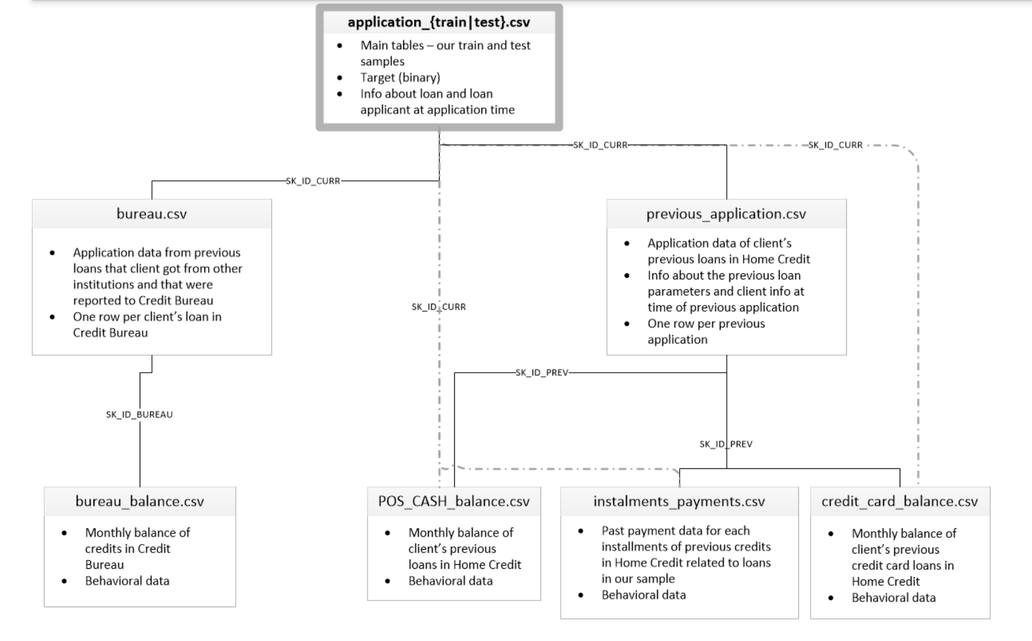
In order to aggregate the data appropriately, we used the following schema to determine the primary and foreign keys necessary for database integration. This allowed us to access all the attributes associated with each customer simultaneously and manipulate the data accordingly.

The first order of business to find which attributes are positively and negatively correlated with our response. We found the following results.

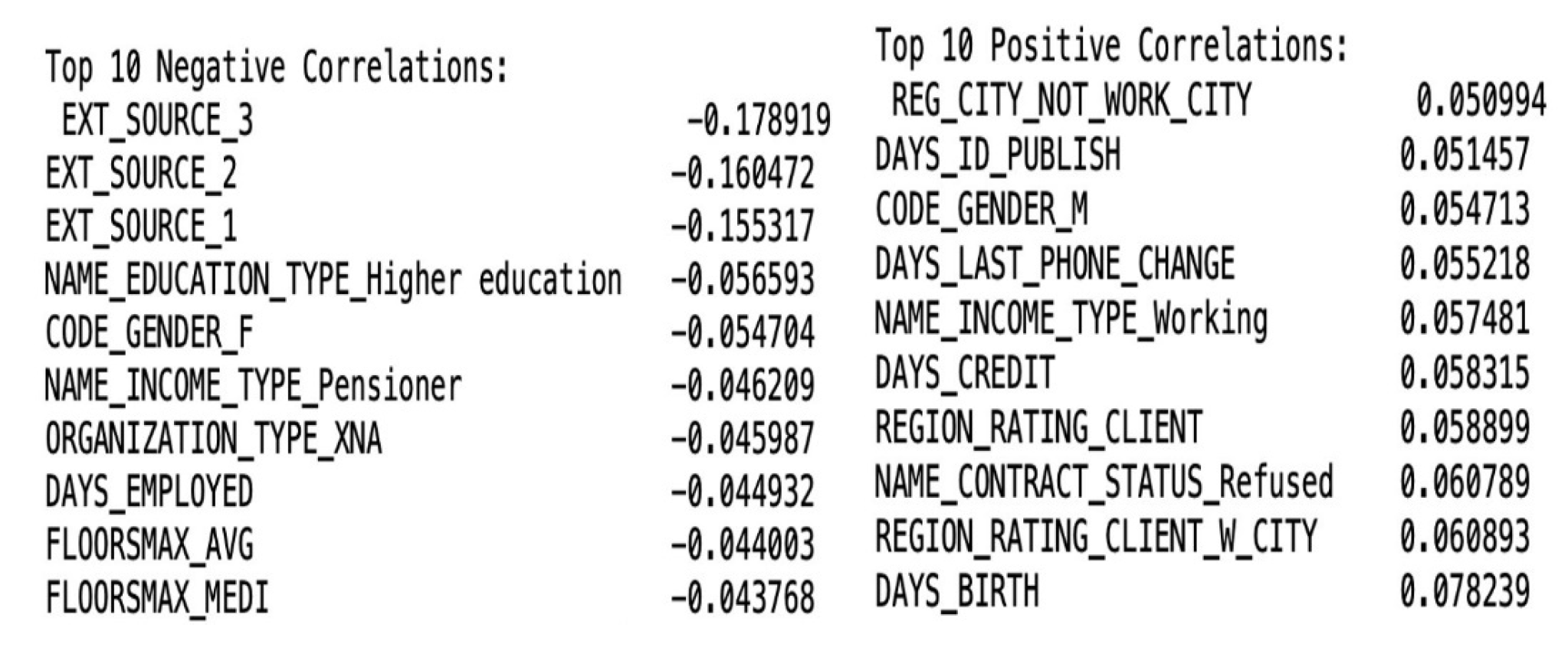
As we can see, the influence of each factor seems incredibly small, but it’s crucial to note the number of factors under consideration during this analysis. Therefore, relatively, this insight is useful. We’ve included part of the myriad of breakdown we’ve built, including the relationships between correlation across age groups, and the variable known as ‘EXT_SOURCE_3’. Upon investigation, we discovered that a large part of the data sourcing comes from confidential financial information that has been tokenized for our use. They’ve been exported into these columns accordingly. This information is insightful particularly because it helps us better predict which attributes, we may observe as a result of our feature selection.

We then wanted to explore whether there were significant correlations between the attributes themselves. We looked through our table with the highest correlations to the response, and then built out heat maps based on their respective values. Since we previously analyzed impact on the target value, we wanted to isolate variables’ relationships to one another. This is particularly insightful to see if there was an aliasing of any kind of variable to one another. If you look at the figure associated with credit card balance, we find that there are a few extraneous highly correlated variables, but their exclusion in our final model did not impact our results, therefore we moved forward with the appropriate feature selection procedures.

2.1.2 Data Cleansing and Feature Selection

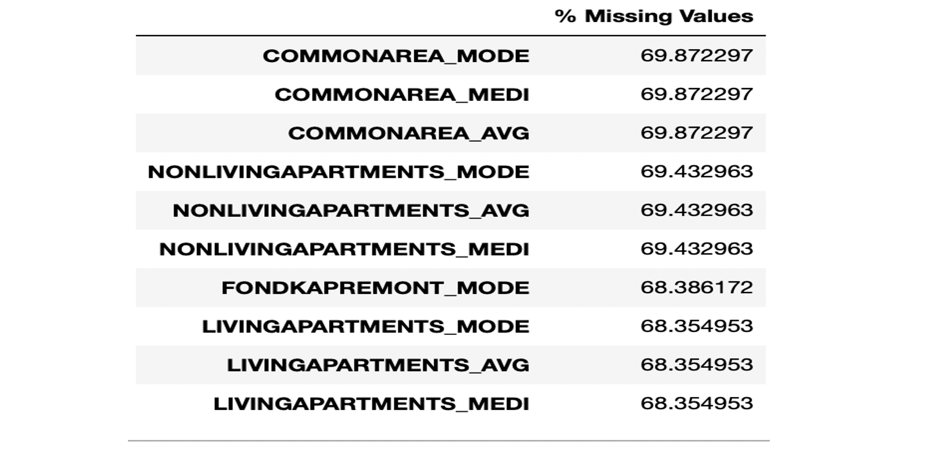
We came across a significant number of columns that had missing values at a proportion that would be misrepresentative to keep in our model. For the columns that had over 60% missing data, we dropped the columns entirely. For those with less than 60%, but still a significant amount of missing data, we used the median of the columns in place of the null values. Here is an example of the list of columns that yielded these results.

In order to prepare our data for feature selection, we needed to identify the datatypes that were utilized and the breakdown of categorical vs quantitative variables. Our analysis displayed the following results.

To make use of the insightful categorical values, we utilized One-Hot Encoding to convert the variables into binary. An example of the conversions as a result of this method are showcased below.

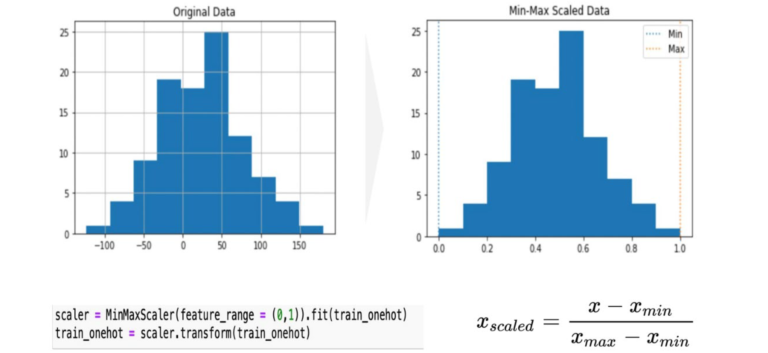
To gauge the accuracy of the conversions and ensure the distribution of values was not skewed in any way, we used minimax standardization. This verifies that all the previously categorical data was on the same scale and that certain variables do not have more of an effect than others. Our results behaved as expected as can be seen below.

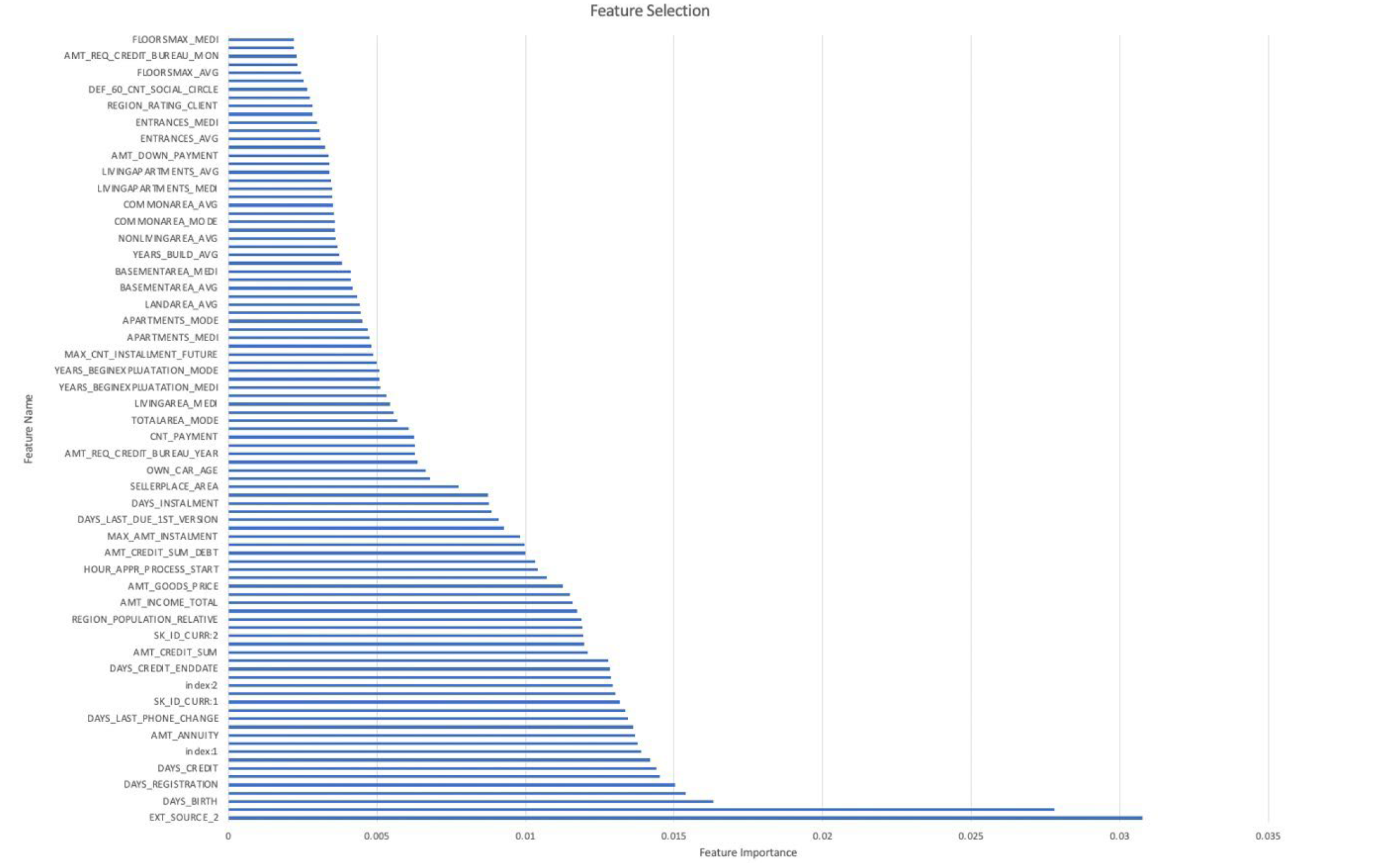
Lastly, we used Random Forest to conduct our final form of feature selection. We finalized on this algorithm after much research for feature selection methods as Random Forest an embedded method meaning the combine the qualities of filter and wrapper method. As a result, they are highly accurate, generalize better, and are interpretable. Due to the nature of the algorithm, they are less prone to overfitting and can more accurately determine the importance of features. After running our algorithm, we were able to finalize on ~70 noteworthy columns as opposed to the previous ~400. Their respective proportion of importance is also displayed.

2.2 Logistic Regression

Logistic regression was used to assess the initial classification task of the data and feature set. We noticed that this algorithm takes a longer time with the large dataset present and had high memory usage. The accuracy produced was 0.919266 with a low AUC score of 0.5026. The possible reasons for low AUC may be due to the assumption that there is a linear relationship between the features and the target variable. If this assumption is not met, the model may not be able to accurately predict the target variable, leading to a low AUC.

2.3 LightGBM

The data exploration process shows that the home credit default risk is large and complicated. Hence, we decided to use the LightGBM model to train our data. LightGBM is a gradient-boosting framework that uses tree-based learning algorithms, which can train data at a faster speed with lower memory usage and is capable of handling large-scale data.

To have a first glance at the LightGBM model, we followed the rule from LightGBM documentation and assign the parameter arbitrarily. The documentation suggests assigning larger max_bin and num_leaves parameters and a smaller training rate for gaining better accuracy. We also assign the feature selection parameter to 0.8 to avoid overfitting. The following image is the first model we made and got a rather good accuracy about 0.903527. Then we investigated the relationship between each parameter and the accuracy. In order to optimize the hyperparameter, we extract the range where the highest accuracy occurs.

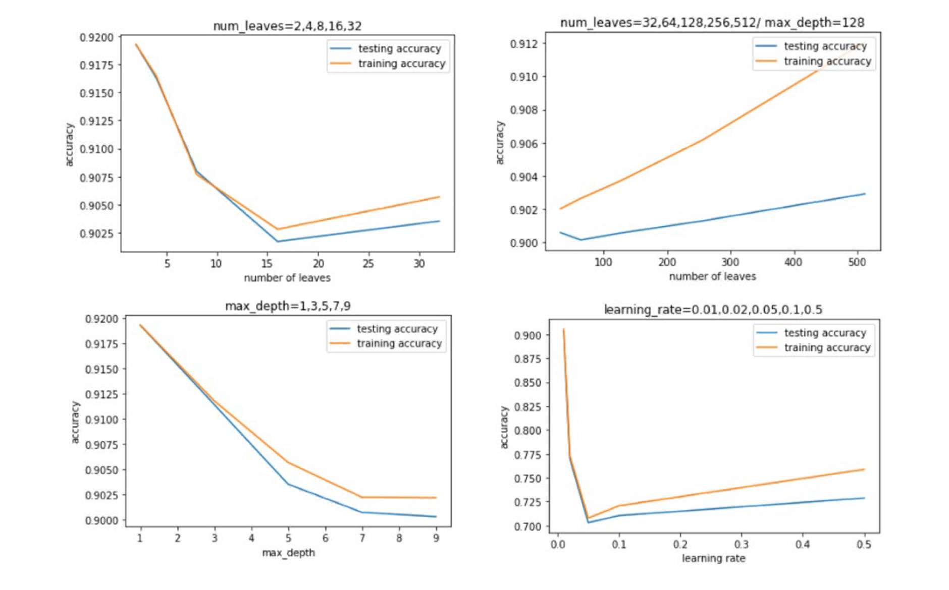
From the graph above, we can observe that the three parameters have similar patterns. We got the highest training and testing accuracy when the parameter value is small. Although both accuracies will increase again as the parameter becomes larger, the gap between training and testing accuracies raise as well, which means overfitting happens. Accordingly, the best range of the number of leaves, maximum depth, and the learning rate is 0 to 5, 0 to 5, and 0 to 0.1 respectively.

After that, we selected some values in the range to find the best combination of parameters that can build the model with the highest accuracy. We imported the GridSearchCV package to help us fulfill this work, and we can see the best combination is to set num_leaves=2, max_depth=1, and learning_rate=0.01. We then utilized these parameters to build the LightGBM again and got a higher accuracy, 0.919266.

3. Results and Discussions

Since the data available to us is an Imbalanced Dataset, we cannot simply use Accuracy as a metric for evaluating the performance of the model. There are some metrics that work well with imbalanced datasets, of which we will use the below-mentioned metrics. The AUC Score insensitive to class imbalance. It works by ranking the probabilities of prediction of the positive class label and calculating the Area under the ROC Curve which is plotted between True Positive Rates and False Positive Rates for each threshold value. This is because we need to minimize the False Negatives, i.e., the people who were predicted as non-Defaulters by the model but were Defaulters. We do not want to miss out on any Defaulter as being classified as non-Defaulter because the cost of making errors could be very high. LightGBM produced a higher AUC of 0.7529 against the 0.5026 of logistic regression. This shows that the boosting algorithm had better classification than binary classification, logistic regression.

4. Conclusions

The constraints from the datasets noticed were mainly on the Interpretability is partially important for classifying someone as a Defaulter or not. After identifying the business objectives and constraints, data imbalance insensitive machine learning algorithm was chosen. Feature Engineering proved to be more useful than model tuning and stacking. Using these we formulate the following conclusions:

• Some categories are discriminatory between the defaulters and non-defaulters.
• Dataset is imbalanced, some correlated features weren’t affecting the performance of the model.
• Defaulters usually tend to have some behavior which deviate from the normal, and thus, we cannot remove outliers or far-off points, as they may suggest some important Defaulting tendency.
• LightGBM boosted the CV from feature selection, Usage of simple forward feature selection technique with Ridge regression and boosting algorithm like XGBoost, may have a further boost in CV and AUC.

5. Appendix

Group Members:

• Cheng-Wei Huang H.Milton Stewart School of Industrial and Systems Engineering
• Arnovi Moinuddin H.Milton Stewart School of Industrial and Systems Engineering
• Kavya Navaneetha Krishnan Guggenheim School of Aerospace Engineering
• Akpevwe Ojameruaye Colleges of Computing, Business, and Engineering

You can find code file and complete report here: https://github.com/wilsoncwhuang/Home-Credit-Default-Risk You can find source data here: https://www.kaggle.com/competitions/home-credit-default-risk/overview