Walmart Sales Prediction

1. Introduction

1.1 Overview

Revenue forecasting has always been crucial for businesses to prepare for upcoming demands and long-term strategic planning. It provides insights in demand planning, storage space allocation, human resource planning, logistics arrangements, and more. Therefore, business owners often deploy certain data analytics models to simulate outcomes that can capture future trends for their operations. Models used to conduct such a simulation may vary based on its required precision or capability for dynamically adjusting to irregularities, but all models are aiming for similar results. Some common predicting models that utilize machine learning techniques for sales forecasting include linear regression, random forest regressions, extreme gradient boosting (XGBoost), long short-term memory (LSTM) model, ARIMA time series forecasting, and more [1]. In this project, we will be using multivariate linear regression techniques to forecast sales trends for targeted retail stores.

1.2 Subject for Analysis - Walmart Supercenters

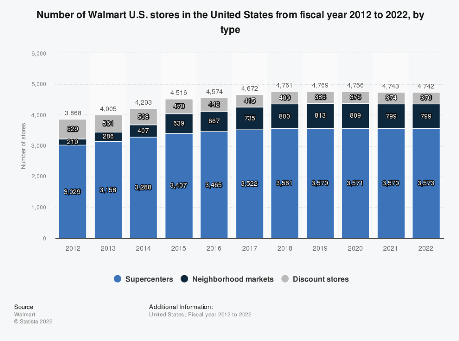
For this project, we will be using regression models to forecast future sales of Walmart Supercenters within the United States. Based on their business model [2], Walmart Supercenters provides a one-stop shopping experience by combining grocery stores with fresh produce, bakery, deli and dairy products. They also include electronics, apparel, toys, and home furnishing items to customers with various needs. Furthermore, most supercenters are open 24 hours with additional services such as banks, hair, pharmacy, and more. The main source of customers for Walmart is from physical retail stores, such as Walmart Superstores, and e-commerce sales. Based on figure 1, we can see that even though the total number of Walmart stores has been slightly decaying, the number of supercenters is still increasing. This indicates the significance of Walmart Supercenters in the United States Region. Therefore, an effective model to forecast future sales for Walmart Supercenters would provide a critical advantage for senior level executives and managers to plan ahead.

2. Problem Statement

In this project, our goal is to predict the weekly sales of Walmart stores based on historical data with several independent variables. Here we selected 10 independent variables that we assume may influence the weekly sales – date, temperature, fuel price, Consumer Price Index, unemployment rate, etc. We further elaborate on these independent and dependent variables as below. One of the biggest challenges for building an effective regression model depends on the quality of selected factors and understanding its correlations between each predictors. As we are curious about what factors may affect the sales revenue of a retail store in the US, we plan to conduct a series of regression analysis with residual analysis and other data validation techniques to find out the most relevant variables. By finalizing these findings, we can better predict the weekly sales with these selected predictors.

3. Data Description

We used the open-source dataset “Walmart Dataset” on Kaggle, the largest data science platform in the world. We got the dataset as a CSV file directly from the URL address: https://www.kaggle.com/datasets/yasserh/walmart-dataset. Our dataset covers the historical sales records and other variables of 45 Walmart stores for the period from 2010/2/5 to 2012/11/1. The sample size of the Walmart Dataset is 6,435. As we split the column Date in the Walmart Dataset into 4 different columns (Year, Month, Day, and Weekday), the number of independent variables will be 10 and the number of dependent variables is 1 in the dataset. In addition, we split the sample dataset into a training set and a test set with an 8:2 ratio (train = 5,148, test = 1,287) to ensure that our prediction is unbiased. Since our current model to obtain the response variable, weekly sales for a specific Walmart store (Weekly_Sales), is a time-dependent study with a 1-week period between each data point, we can assume the data points we use are time-dependent. The following table summarizes the description and categories of our 11 variables:

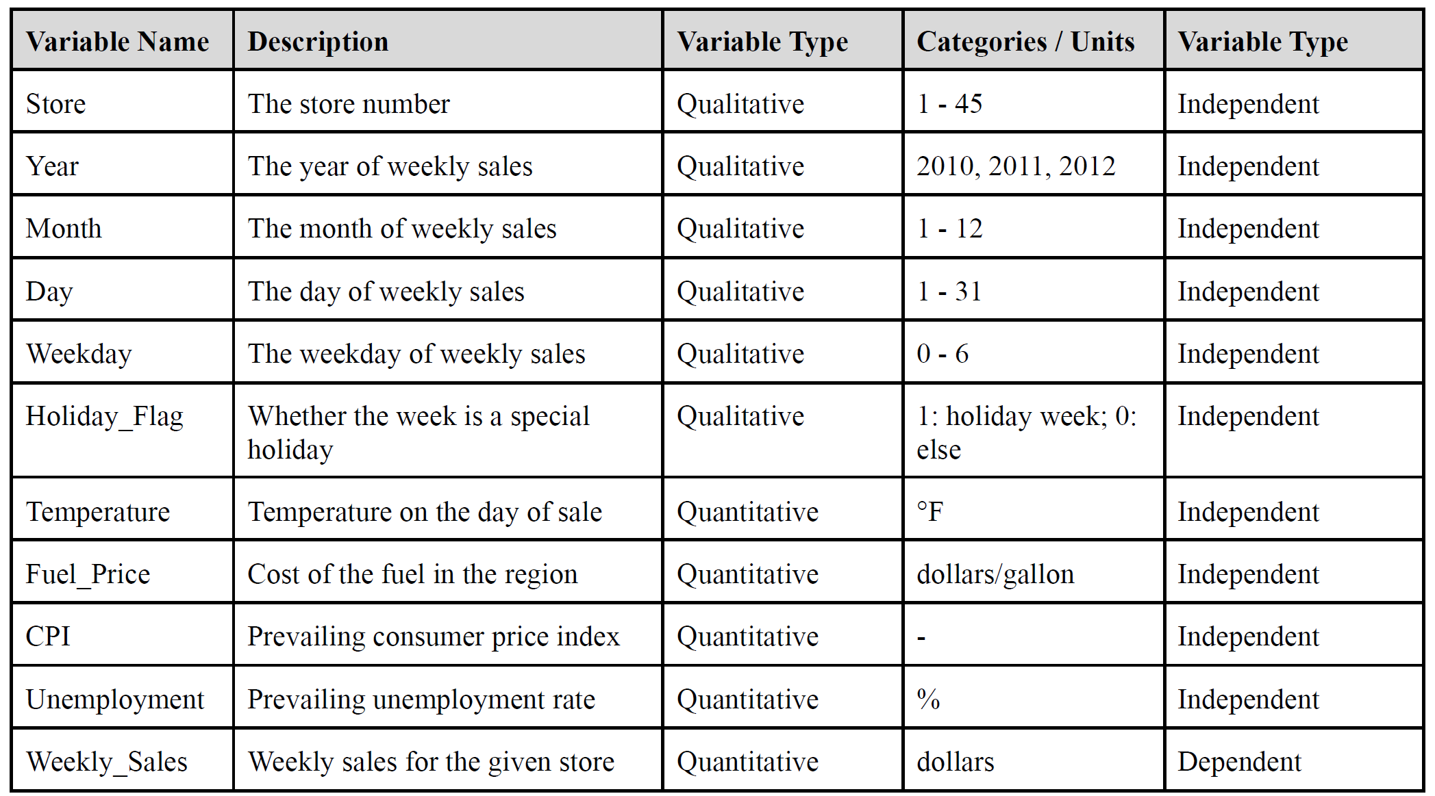
For the qualitative variables, Holiday_Flag can be viewed as a dummy variable that indicates whether a specific data point includes holidays within its period. This variable is related to our assumption that holidays may create a temporary spike in demand, which leads to a higher weekly sales amount for the store. The other qualitative variable is Store, which simply indicates the Walmart store number that is covered in our study. Since the study only includes a certain amount of stores to analyze, the data directly assign each store with a numerical value between 1 to 45 (total Walmart store within the study: 45).

4. Regression Analysis

After basic data preprocessing, we performed the following processes for the regression analysis. First of all, we performed some exploratory analysis on our dataset to see if there are any noteworthy characteristics or trends of the variables. We then built a full multiple linear regression model based on all the predictors we originally have. After analysis and diagnosis, we took different actions on the full model and built several reduced regression models to improve the model performance, and we conducted residual analysis and checked if the basic regression assumptions hold in each of our reduced models accordingly. Finally, we used our test data to conduct predictions on our models.

In the following section, R would be the main tool for our regression analysis.

4.1 Exploratory Analysis

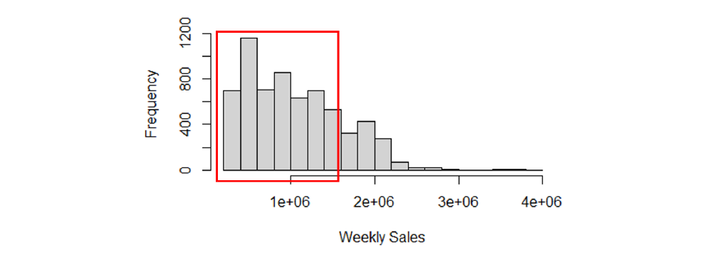
First of all, Figure 2 shows the frequency of the response variable, Weekly_Sales. The weekly sales are around 1 million dollars in most Walmart stores. It implies that the response variable would be in a great range of scale.

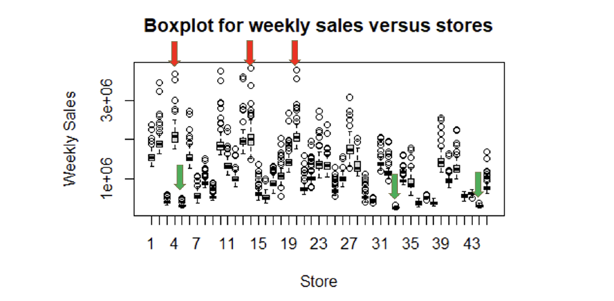
We can see that Store 4, 14, 20 have higher weekly sales with larger variability in Figure 3. On the other hand, the weekly sales are lower in Store 5, 33, 44. This might be caused by the different areas these 45 stores are located.

In Figure 4 below, the average of weekly sales among stores is similar in each month. We notice that there are more data points outside the 75th percentile in December than in other months. It indicates that people would purchase much more in December, the Christmas holiday season.

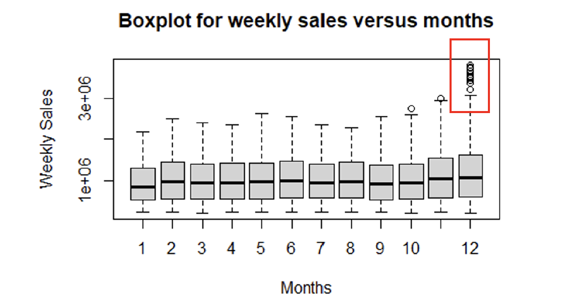
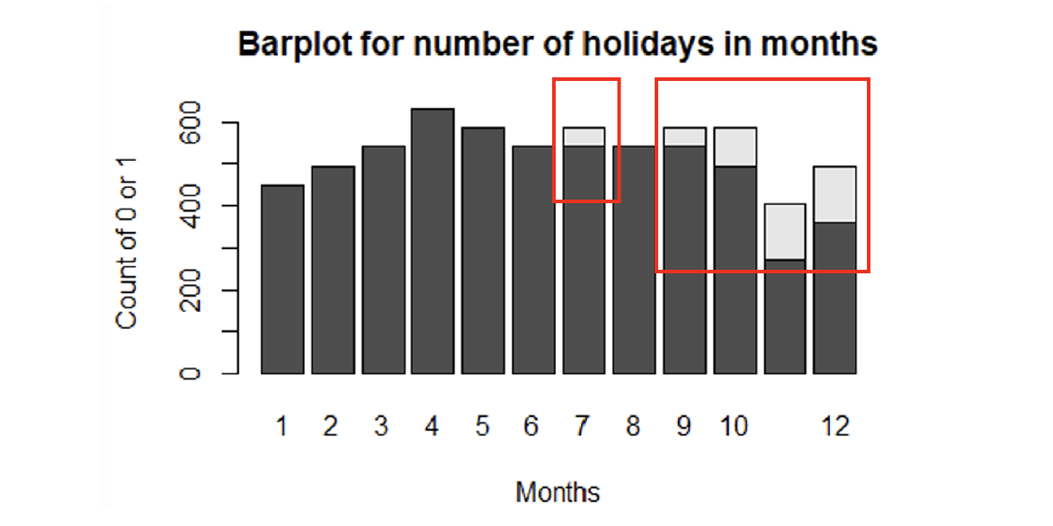
Figure 5 displays that July, September, October, November, and December should be holiday seasons with counts of holiday flags (Holiday_Flag = 1, the white area in the histogram).

4.2 Regression Analysis - Full Model

After preprocessing and exploring the dataset, we built a full linear regression model with all predictors we currently have. The basic information of this model is summarized in the Appendix section - Summary of Full model. We set our significance level at 0.05, and noticed that 16 of the predictors are insignificant in the full model. In addition, the R-squared value is 94.29% and the adjusted R-squared value is 94.18%, which is quite high and may result from multicollinearity. Based on these facts of the full models, we want to further improve our model to enhance its prediction performance. We accordingly performed stepwise regression for feature selection, conducted the residual analysis to test if basic assumptions hold in the model, applied data transformation, identified potential outliers, and checked for multicollinearity. These processes and results are elaborated on in the following paragraphs.

4.3 Forward and Backward Stepwise Regression

In order to avoid potential overfitting issues, we conducted forward and backward stepwise regression to perform feature selection. This is because we got a relatively high R-squared in our full model. From the result in Appendix section - Results of Forward/Backward Stepwise Regression both forward and backward stepwise regression shows that the model with all predictors has the best AIC value. It might be because we split the testing from our original data, which might be very clean initially.

4.4 Residual Analysis - Full Model

4.4.1 Linearity Assumption

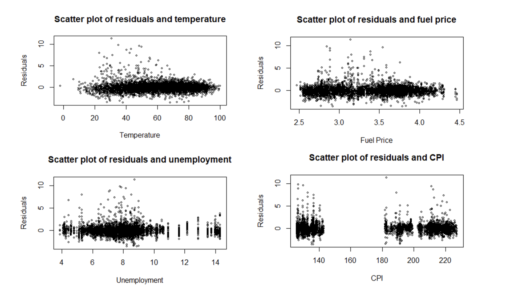
The scatter plots below show the standardized residuals against each quantitative variable, Temperature, Fuel_Price, Unemployment, and CPI. The data points are randomly scattered around 0. This shows that the Linearity assumption holds for the full model.

4.4.2 Constant Variance Assumption

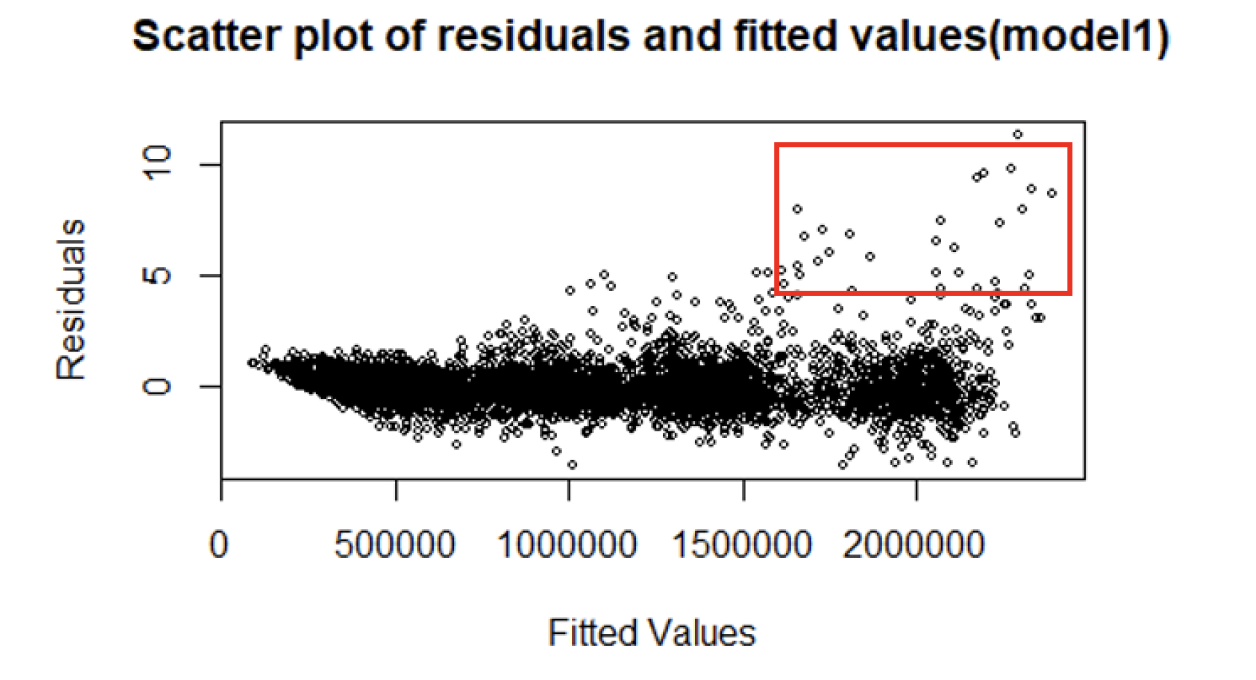
Overall, the plots are scattered randomly around 0 in Figure 7. However, a few standardized residuals show larger variance as the predicting variable increases. The constant variance assumption might not hold for the complete model.

4.4.3 Normality Assumption

The histogram of the standardized residuals for the full model is bell-shaped in the left chart of Figure 8. It shows that the residuals should have an approximately symmetric and unimodal distribution. However, the curvature at the ends of the Q-Q plot on the right of Figure 8 suggests a non-normality in the complete model.

4.5 Outlier Checks - Full Model

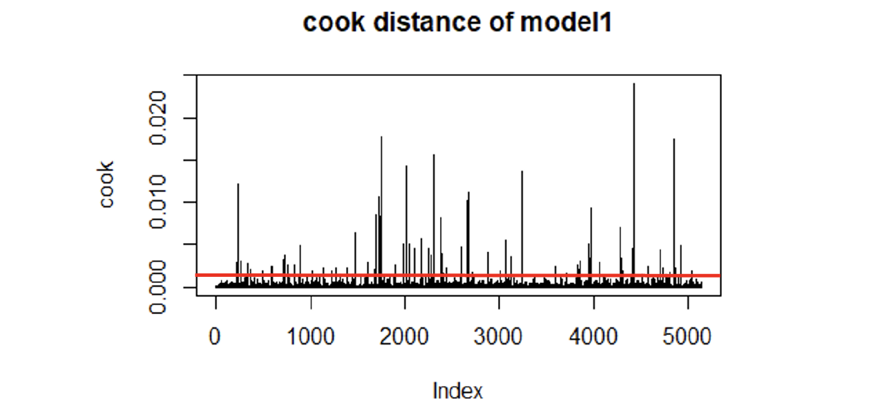
We conducted Cook’s Distance as a measure to exclude the outliers. The threshold we selected is 0.0078, retrieved from 4 divided by the size of the sample dataset (=4/5148). In Figure 9, there are several data points that should be removed from this criteria.

4.6 Multicollinearity Diagnosis - Full Model

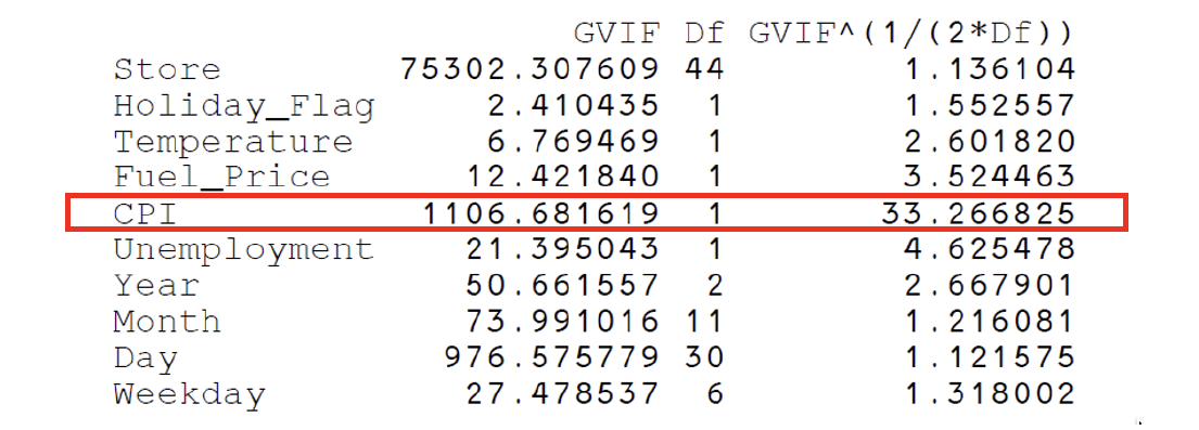
For VIF (Variance Inflation Factor) analysis, we would like to take the degree of freedom into account for our model since the number of categories for the qualitative variables is relatively large in the data set. The result shown in Figure 10 indicates that the VIF value of CPI is significantly higher than other predicting variables. This suggests that CPI might be more correlated with the other predictors. Thus, it should be taken out potentially.

4.7 Improvements - Reduced Model

Based on the residual analysis, outlier checking, and multicollinearity diagnosis presented in the previous sections, we performed 3 improvements to acquire a better model.

1. Fitted the model with Square Root Transformation. We plan to eliminate the violation of assumptions by fitting the model with square root transformation.
2. Removed the outliers with Cook’s Distance larger than 0.0078. If there are a large number of outliers, they probably point to a heavy tailed distribution rather than truly extreme values. To fix the assumption violation issue, the outliers would be taken away.
3. Removed the predictor CPI. We would like to improve R-Squared by excluding the predictor that is correlated with the other predictors potentially.

We built the additional 7 models based on the different combinations among the 3 measures. Also, we performed predictions on our test dataset with these models. The result will be explained further in the next section.

4.8 Models Comparison

According to the above assumptions, we combined three different improvements and then generated 8 different models. To compare these models, we calculated adjusted R-squared and R-squared to analyze the residuals of training data and calculated MSPE and precision measure to see the reliability of prediction.

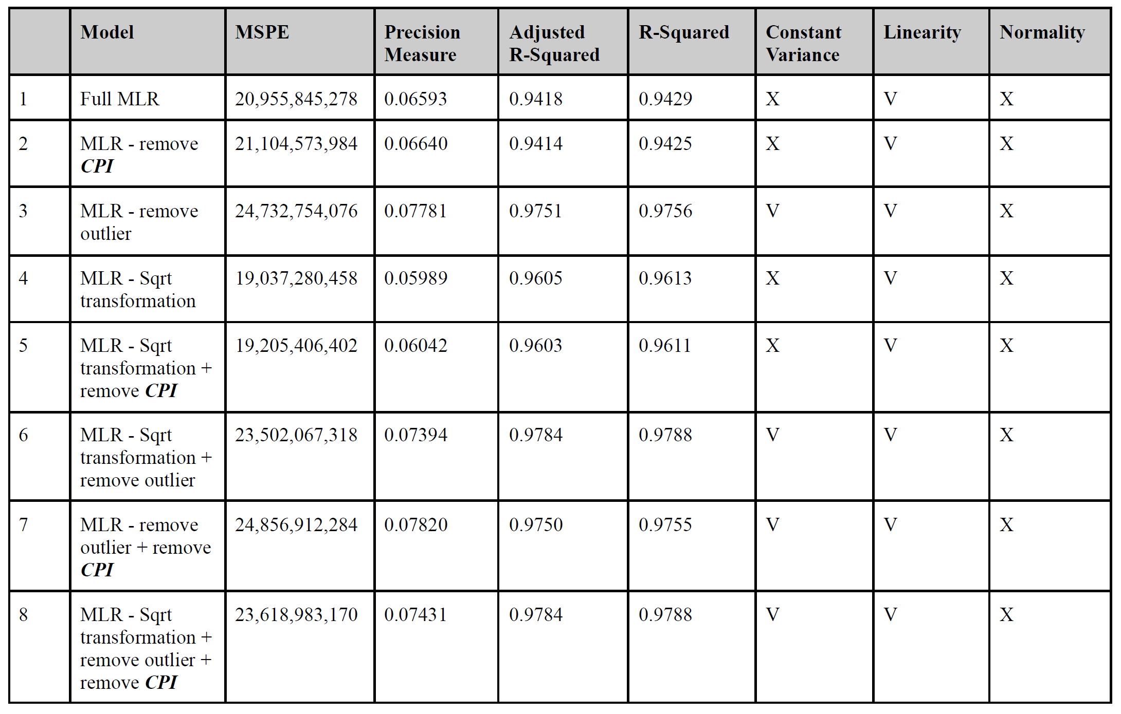
From the above table, we can observe that the 7th (remove outlier and CPI) model has the best R-squared value. However, its MSPE value is significantly larger than the 4th (squared transformation) and 5th (squared transformation and remove CPI) models. In contrast, although the 4th model’s R-squared is not as high as the 7th model, it has the lowest MSPE among the 8 models, which means it has the least chance to cause an overfitting issue. We therefore chose the 4th model to be our final selected model.

We also test the model for three multiple linear regression assumptions. We can see that all models follow the linearity assumption and violate the normality assumption. As for the constant variance assumption, which only holds in models that outliers are removed. Though some of the models after modification or transformation still violate the variance assumption, the new models perform much better in these assumptions than the full model. The plots of the three assumptions for all models except the full model and the final selected model can be found in the appendix.

4.9 Summary of Final Selected Model

From the summary table of the final selected model (Model 4) in Appendix section - Summary of Reduced Model Model 4, we can find the statistically insignificant and significant variables based on 95% confidence level.

4.10 Linearity, Normality, and Constant Variance Assumption of Final Selected Model

The above plots show that the final selected model follows the linearity assumption, and violates the normality and constant variance assumption. However, the variance of residuals is smaller than the full model.

5. Conclusions and Recommendations

5.1 Final Selected Model

In summary, we choose the multiple linear regression model with the square root transformation (model 4) to be our suggested final model, based on the fact that it has the lowest MSPE among the 8 models while maintaining a decent R-squared value. We believe that Walmart can apply this model for future weekly sales prediction and use it to foresee any seasonal and promotional demand spikes.

However, as the normality assumption does not hold in any of the models we built, further evaluation may be conducted to check the reason behind this situation when applying the model.

5.2 Recommendations for Improvement

Based on the regression model selected, we can predict weekly sales for individual stores at certain locations in the United States with certain economic, environmental, and seasonal factors. Even though the current model already demonstrates a certain level of accuracy toward the collected dataset, several recommendations could still be made to improve the adaptability and accuracy of our regression model:

1. Longer time frame

In the current training dataset, our time frame covers 2 years of data ranging from 2010 to 2012. Two years of data may be sufficient to predict weekly sales at a relatively stable year with only a few anomalies. However, after experiencing the pandemic in 2020 and other economic depression from recent years, these supply chain disruptions should be considered in the model for a more up-to-date result. For example, Fuel price and unemployment rate around the pandemic era (2020 to 2021) experience significant fluctuations. These influences should either be collected into the current dataset or to build a contingent model with consideration of abnormal economic events.

2. Include additional store locations

Based on our current dataset, we have data from a total of 45 Walmart supercenter locations within the United States. Since our data was provided based on a credible third-party contributor on Kaggle, we have minimal capability to identify the actual geographic locations of the represented stores in our data. In future research stages, it is recommended to add additional store locations that cover a more holistic demographic throughout the United States. The dataset can also include region information (i.e midwest, west coast, east coast, etc.) to include regional effects to weekly sales forecast. This improvement can result in a more comprehensive model for Walmart to predict sales in different regions.

3. Product categories as predictors

Weekly forecast as our response variable demonstrates the overall weekly sales trend and other high-level information. However, to actually provide an actionable plan for Walmart supercenters to prepare future demands, specific product or product categories should be included as one of the predicting variables. This information is crucial for supply chain or store managers to plan ahead. Managers can target specific product categories to stock in advance for potential demand spike due to certain factors. This information will not only be useful for predicting holiday demands but also prepare for demand fluctuations on certain types of product when economic indicators fall below a predefined threshold.

4. Operating and labor costs

As mentioned above, the weekly sales response variable captures the overall sales data of Walmart supercenter. To increase the usability of the data, we could incorporate the operating and labor costs for each Walmart supercenter to obtain the weekly profit for a more direct performance measurement. For example, operating costs such as weekly utility spendings, equipment spendings, and other technology enhancements could play an important role in averaging out sales spikes in certain situations. For human labor on the other hand, since it is a recurring cost for every month, the effects on weekly sales may be a systematic difference depending on the operating situation in each store. In summary, these spending information are critical to evaluate the current profit of each Walmart location and provide insight for managers to understand the reality of their sales performances.

6. Reference

[1] Liebeskind, M. (2021, December 14). 5 Machine Learning Techniques for Sales Forecasting. Medium. link

[2] About Walmart. (n.d.). Corporate - Walmart US. link

7. Appendix

Group Members:

• Cheng-Wei Huang H.Milton Stewart School of Industrial and Systems Engineering
• Jyh-Heng Yu H.Milton Stewart School of Industrial and Systems Engineering
• Chin-Heng Lin Colleges of Computing, Business, and Engineering
• Yu-Ching Chen Colleges of Computing, Business, and Engineering

You can find code file and complete report here: https://github.com/wilsoncwhuang/Walmart-Sales-Prediction